Speed comparisons

Here, I compared the performance of rtrees (v1.0.0) and V.PhyloMaker (v0.1.0) (V.PhyloMaker2 has almost the same speed as V.PhyloMaker, so no comparisons here). In most cases, rtrees is at least two times faster than V.PhyloMaker (Fig. below). For example, with 50 missing species to bind, the average time used by rtrees is 0.914 second while V.PhyloMaker took 13.6 seconds on average; with 5,000 missing species to bind, rtrees used 80.9 seconds on average while V.PhyloMaker used 187 seconds. In general, the time used by rtrees and V.PhyloMaker increased 15.6 and 34.8 seconds on average with 1,000 more missing species to be grafted, respectively. All tests were conducted on a 14’ Macbook Pro with M1 pro chip.

Some may not think it is a big difference. However, for me as a user, waiting for more than 10 seconds to have about 50 species grafted is not ideal. Also the accumulated time can be large if one is doing this multiple times (e.g., doing some simulations that require thousands of iterations).

The R code used for the speed tests can be found here.

if(!require("ggplot2")) install.packages("ggplot2")
#> Loading required package: ggplot2
library(ggplot2)
# library(broom)
temf = tempfile()
download.file("https://raw.githubusercontent.com/daijiang/rtrees_ms/main/Data/rtrees_speed_out.rds", 
              destfile = temf)
speed_out = readRDS(temf)
speed_out = dplyr::mutate(speed_out, n_sp_missing_k = n_sp_missing / 1000, time_s = time/1e9)
# speed_lm = dplyr::group_by(speed_out, expr) |> 
#   dplyr::do(broom::tidy(lm(time_s ~ n_sp_missing_k, data = .))) |> 
#   dplyr::ungroup()
ggplot(speed_out, aes(x = n_sp_missing_k, y = time_s, color = expr, group = expr)) +
  geom_point() +
  geom_smooth(method = "lm") +
  labs(x = "Number of binding species (Thousand)",
       y = "Time (Second)", color = NULL, group = NULL) +
  scale_x_continuous(breaks = c(0.05, seq(0.5, 5, 0.5))) +
  scale_y_continuous(breaks = c(0, 10, seq(25, 200, 25))) +
  geom_text(x = 4, y = 33, label = "rtrees: y = -0.09 + 15.6x", inherit.aes = FALSE, color = "#F8766D") +
  geom_text(x = 1.8, y = 123, label = "V.PhyloMaker: y = 11.80 + 34.8x", inherit.aes = FALSE, color = "#00BFC4") +
  theme(legend.position = "none") 
#> `geom_smooth()` using formula = 'y ~ x'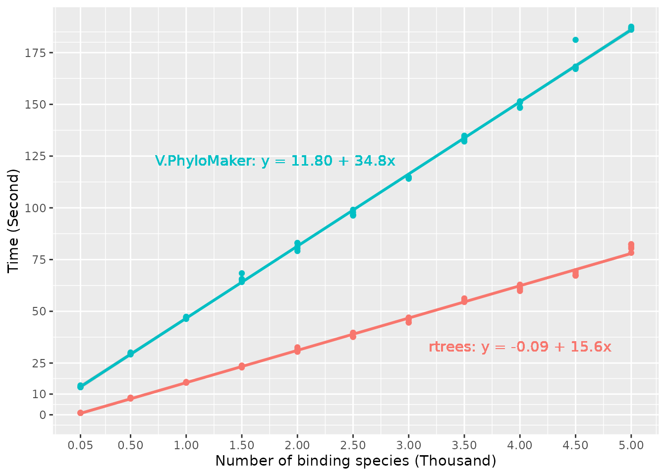

Based on the figure above, the time used by rtrees (and other R packages such as V.PhyloMaker and FishPhyloMaker) increased linearly with the number of missing species. This is because of the sequential structure of the R phylo object, in which all tips and nodes of a phylogeny are labeled with continued integers. When a new node or tip needs to be inserted, all the numbers after the binding location need to be pushed one place after. Therefore, the binding of tips in an R phylo object is a sequential process, which cannot be conducted with parallel computing to take advantage of the multiple CPU cores a regular computer has nowadays. It is possible to speed it up by converting some core R code into C++. However, it takes a lot of effort to do this right.

Another potential resolution is to represent phylogenies in a non-sequential structure unlike phylo objects in R. One example is the treeman package, which developed such a structure to perform tree manipulations. Because of the non-sequential structure (i.e., no continuous labeling of nodes and tips), it is possible to use parallel computing to process phylogenies. However, such a structure has not yet been adapted widely by the R community. Therefore, the infrastructure to support such a non-sequential structure in R is still missing, making it hard to use it here in rtrees.

Despite the limitations described above, rtrees is reasonably fast and user-friendly with informative messages.